PlotPub-v2.0 Documentation
Contents
Tutorial
NOTICE: Tutorial for v1.4 is here.
To create a beautiful figure using PlotPub, all you need to know is how to use the (Plot) class. Alternatively, you can use the set-plot-properties (setPlotProp) function which is discussed here. The Plot class provides a simple and elegant object oriented programming interface for manipulating MATLAB figures.
Let us walk you through an example. Assume that we have data for 3 cycle of a 50 Hz AC voltage signal:
clear all;
%% lets plot 3 cycles of 50Hz AC voltage
f = 50; % frequency
Vm = 10; % peak
phi = 0; % phase
% generate the signal
t = [0:0.0001:3/f];
th = 2*pi*f*t;
v = Vm*sin(th+phi);
% plot it
figure;
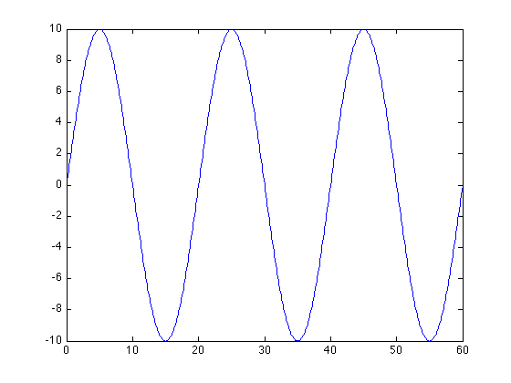
plot(t*1E3, v);
where, f is the frequency, Vm is the peak voltage, t is time and v is the AC voltage signal. Result? An utterly ugly looking figure punching at your face:
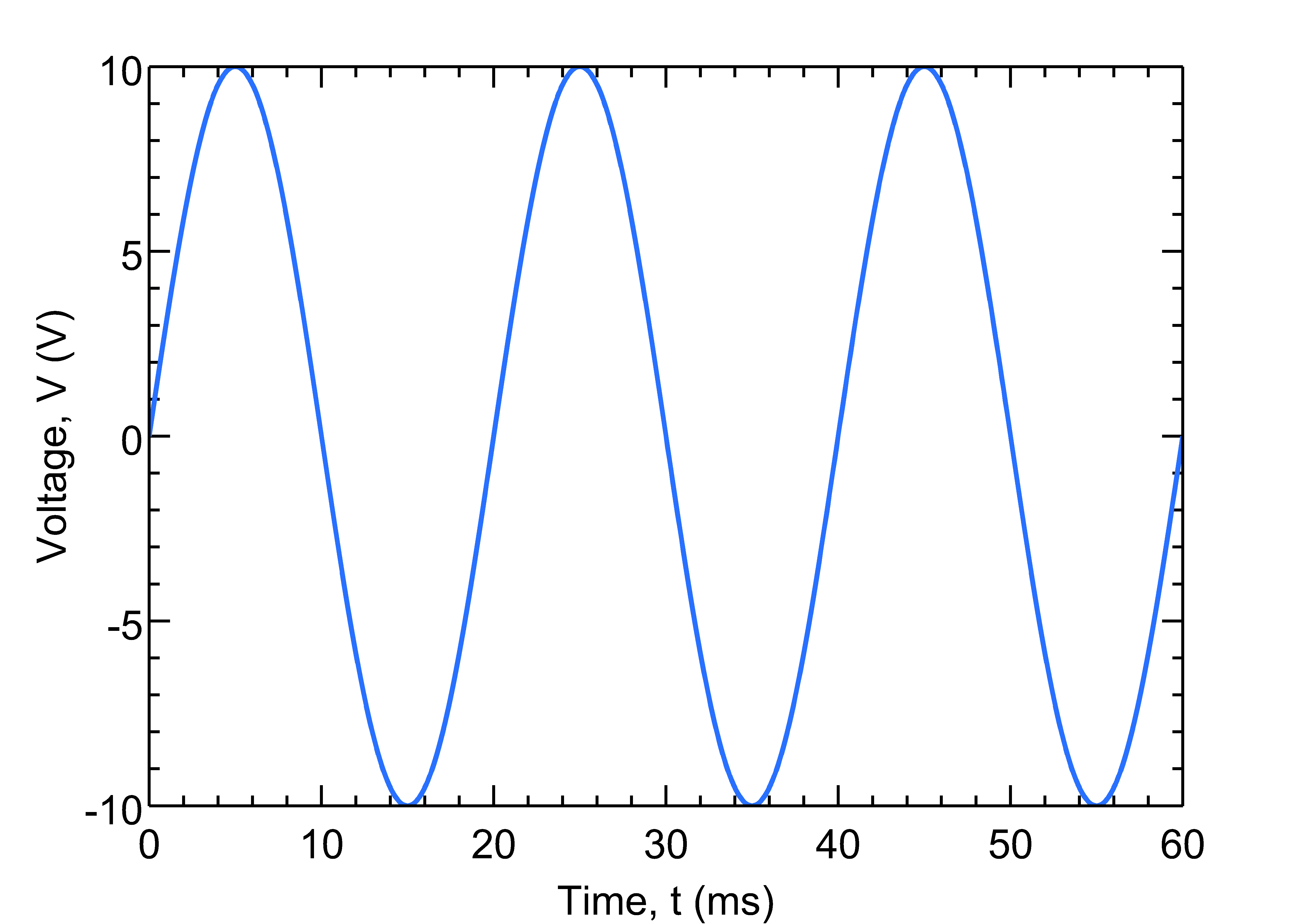
Now, let us add some spices. Let us set the labels and title:
% change settings
plt = Plot(); % create a Plot object and grab the current figure

plt.XLabel = 'Time, t (ms)'; % xlabel
plt.YLabel = 'Voltage, V (V)'; %ylabel
plt.Title = 'Voltage as a function of time'; % plot title
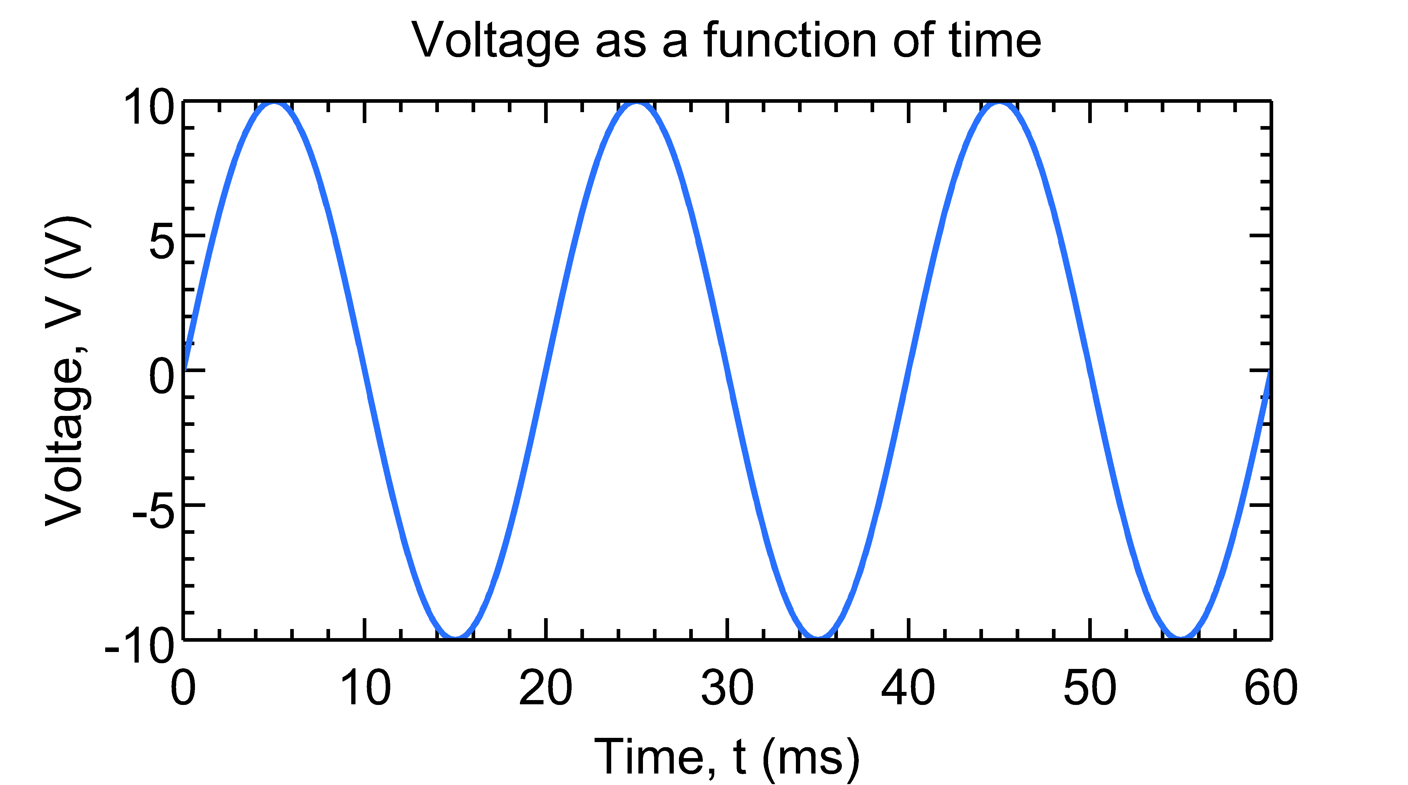
Finally, call the export function to export the figure:
% Save? comment the following line if you do not want to save
plt.export('plotSimple1.png');
The resulting plot should look like:
Instead of creating the plot using:
% plot it
figure;
plot(t*1E3, v);
one could also use Plot class directly to plot:
plt = Plot(t*1E3, v); % create the figure directly using data

plt.XLabel = 'Time, t (ms)'; % xlabel
plt.YLabel = 'Voltage, V (V)'; %ylabel
plt.Title = 'Voltage as a function of time'; % plot title
The full source code for this plot, plotSimple.m, can be found inside the examples_class folder.
We can change color, linewidth, linestyle etc:
plt.Colors = {[0, 0, 0]}; % [red, green, blue]
plt.LineWidth = 2; % line width
plt.LineStyle = {'--'}; % line style: '-', ':', '--' etc
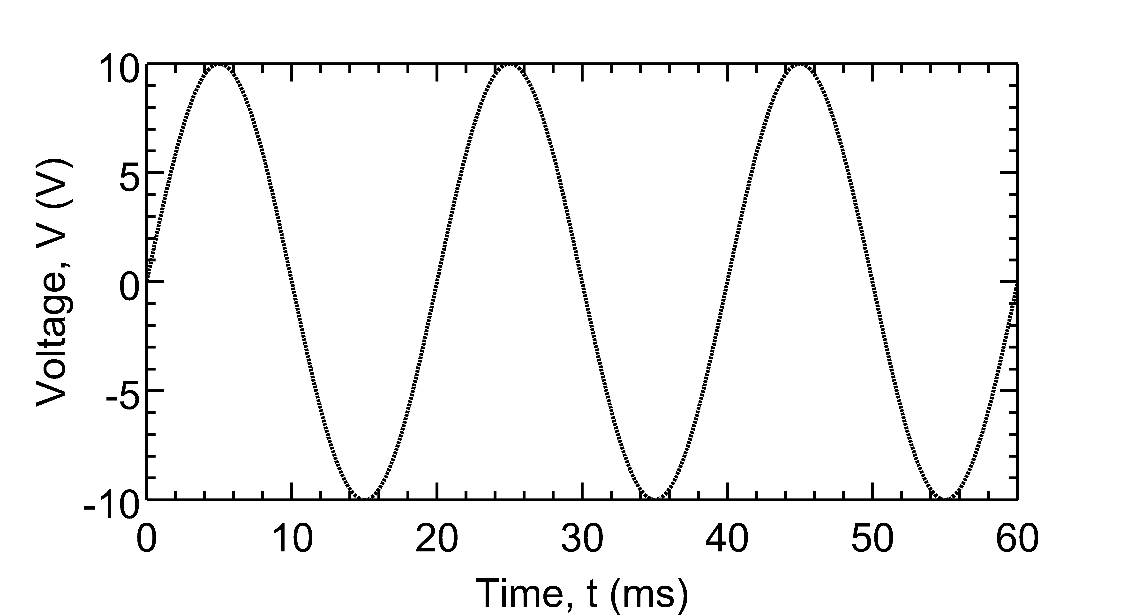
See plotLineStyle.m for full source code.
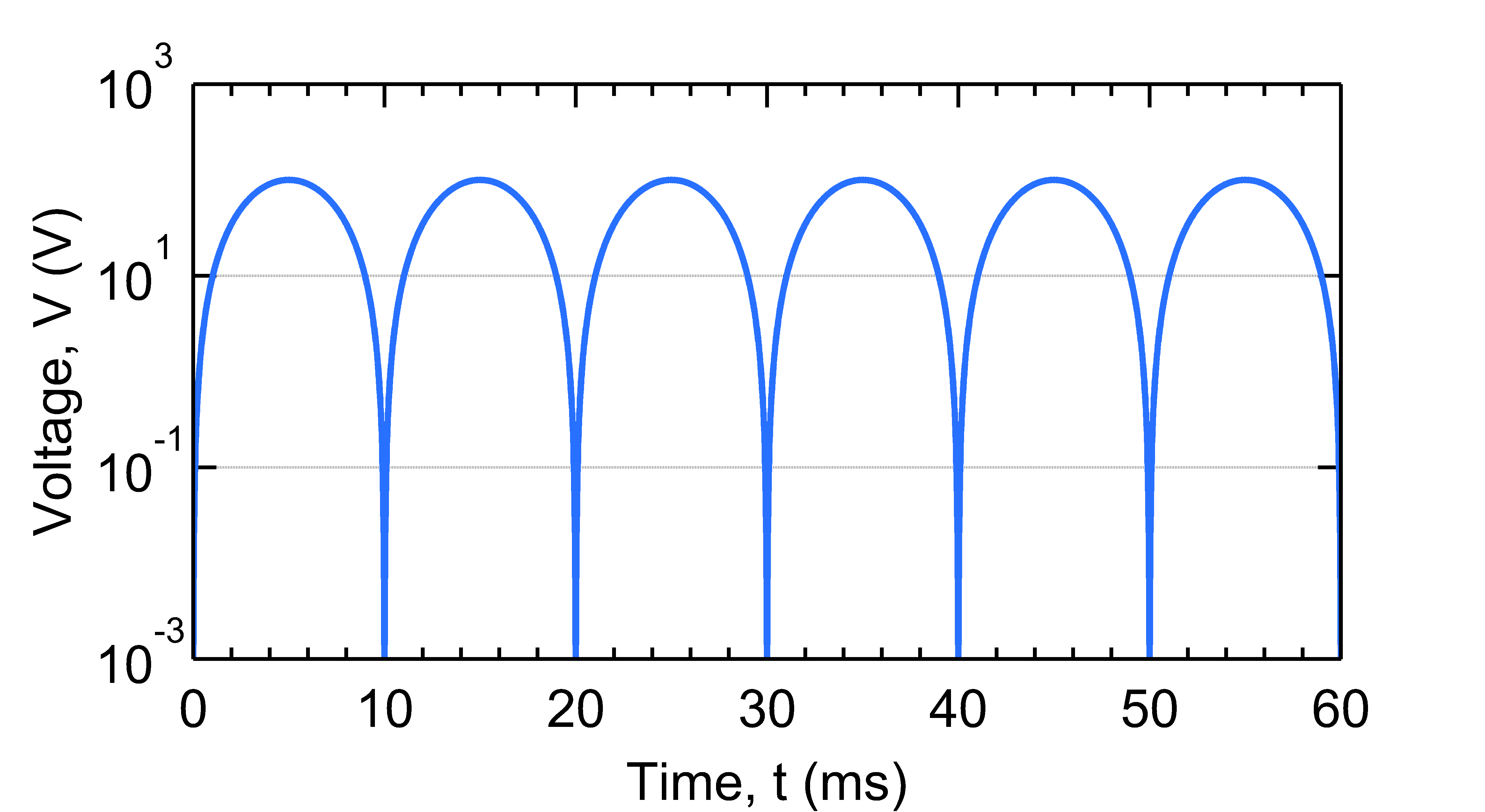
We can also change scale, axis limit, tick and grid:
plt.YScale = 'log'; % 'linear' or 'log'
plt.YLim = [1E-3, 1E3]; % [min, max]
plt.YTick = [1E-3, 1E-1, 1E1, 1E3]; %[tick1, tick2, .. ]
plt.YGrid = 'on'; % 'on' or 'off'
or create a log-log plot:
plt.YScale = 'log'; % 'linear' or 'log'
plt.XScale = 'log'; % 'linear' or 'log'
plt.YLim = [1E-3, 1E3]; % [min, max]
plt.YTick = [1E-3, 1E-1, 1E1, 1E3]; %[tick1, tick2, .. ]
plt.YGrid = 'on'; % 'on' or 'off'
plt.XGrid = 'on'; % 'on' or 'off'
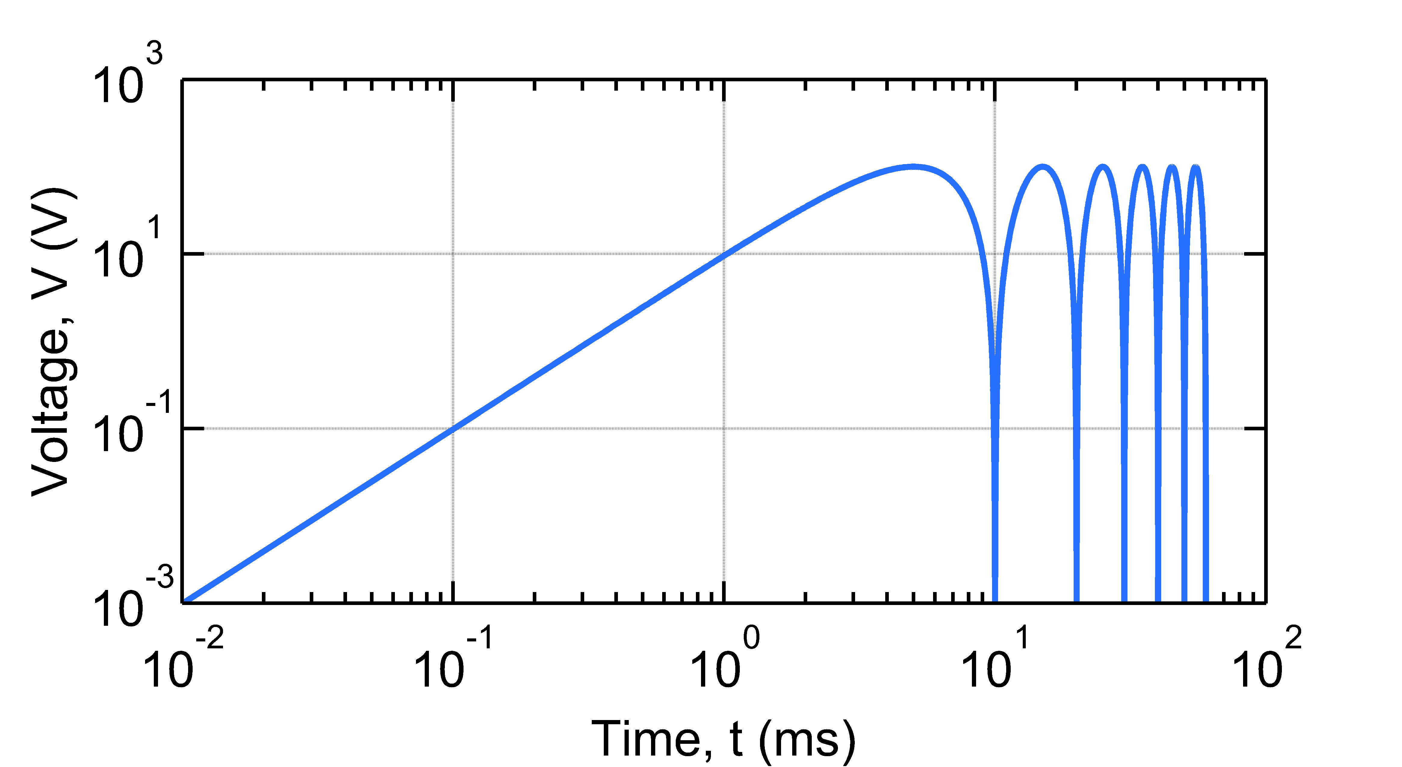
See plotSimpleLog.m and plotSimpleLogLog.m for full source code.
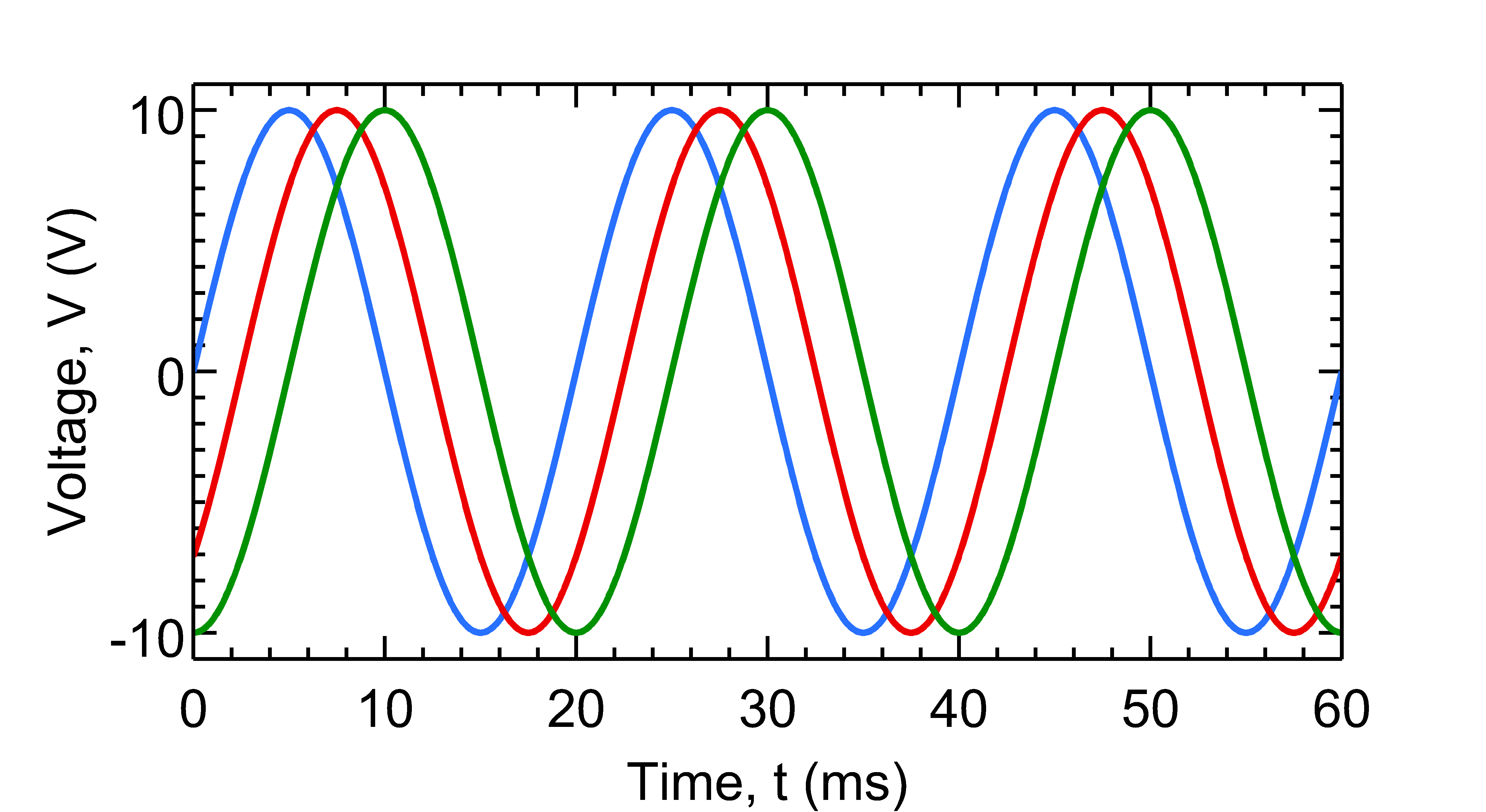
Creating multiple plots in a single set of axes is also easy:
% generate the signal
t = [0:0.0001:3/f];
th = 2*pi*f*t;
v1 = Vm*sin(th);
v2 = Vm*sin(th - phi);
v3 = Vm*sin(th - phi\*2);

% plot them
plt = Plot(t*1E3, v1, t*1E3, v2, t*1E3, v3);

% change settings
plt.XLabel = 'Time, t (ms)'; % xlabel
plt.YLabel = 'Voltage, V (V)'; % ylabel
plt.YTick = [-10, 0, 10]; % [tick1, tick2, .. ]
plt.YLim = [-11, 11]; % [min, max]

% Save? comment the following line if you do not want to save
plt.export('plotMultiple.tiff');
Note how Plot class constructor is directly used for plotting multiple functions. Result:
The full source is given in plotMultiple.m. We can change the linestyle, color etc and add a legend:
plt.XLim = [0, 80]; % [min, max]
plt.Colors = { % three colors for three data set
    [1, 0, 0] % data set 1
    [0.25, 0.25, 0.25] % data set 2
    [0, 0, 1] % data set 3
};
plt.LineWidth = [2, 2, 2]; % three line widths
plt.LineStyle = {'-', '-', '-'}; % three line styles
plt.Markers = {'o', '', 's'};
plt.MarkerSpacing = [15, 15, 15];
plt.Legend = {'\theta = 0^o', '\theta = 45^o', '\theta = 90^o'}; % legends
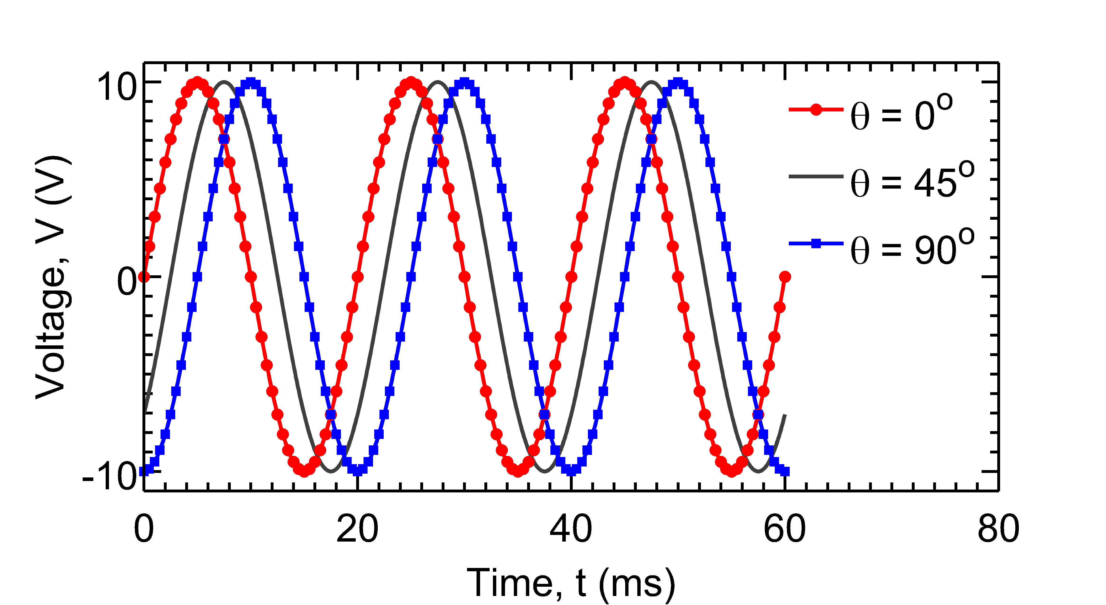
Here, plt.Colors{1}, plt.LineWidth(1) and plt.LineStyle{1} set properties of data set 1 and so on. The full source is given in plotMarkers.m.
By default, PlotPub creates figures with 6in x 3in box size. You can easily change the figure size using the following code.
plt.BoxDim = [7, 3]; %[width, height] in inches
This code creates a figure with 7in x 5in box.
See plotSize.m for more details.
You can also load a previously saved MATLAB fig file and export it using Plot class:
clear all;

% load previously generated fig file
plt = Plot('single.fig');

% change settings
plt.XLabel = 'Time, t (ms)'; % xlabel
plt.YLabel = 'Voltage, V (V)'; %ylabel
plt.BoxDim = [6, 5]; %[width, height]

% Save? comment the following line if you do not want to save
plt.export('plotSize.png');
Reference Manual
Manual for v1.4 is here.
Given bellow is a brief description of the Plot class and setPlotProp and plotPub functions and their parameters. This documents can also be viewed by invoking:
>> help Plot
>> help setPlotProp
from inside the MATLAB command window.
The Plot class
This class represents a MATLAB figure. It can create new plots, open saved figure files and change properties of opened/existing figures. It can also export figures as publication quality image files. The resolution of the image can be changed by the user. Supported image formats are EPS, PDF, PNG, JPEG and TIFF. The figure properties can be changed by easy-to-remember class properties.
Constructors
Plot()
% Grabs the current figure.
Plot(handle)
% Grabs the figure pointed by handle.
Plot('filename.fig')
% Opens the figure file ('filename.fig') and use the opened figure.
Plot(handle, holdLine)
% Grabs the figure pointed by handle. If holdLine = true, it does not
% change the plot properties.
Plot(Y)
% Plots Y where Y must be a vector.
Plot(X, Y)
% Plots Y vs X. Both X and Y must be vectors.
Plot(X1, Y1, X2, Y2, ...)
% Plots Y's vs X's. X's and Y's must be vectors.
The constructors return plot objects which can be used for subsequent property changes.
Properties
BoxDim % vector [width, height]: size of the axes box in inches;
% default: [6, 2.5]
ShowBox % 'on' = show or 'off' = hide bounding box
FontName % string: font name; default: 'Helvetica'
FontSize % integer; default: 26
LineWidth % vector [width1, width2, ..]: element i changes the
% property of i-th dataset; default: 2
LineStyle % cell array {'style1', 'style2', ..}: element i changes
% the property of i-th dataset; default: '-'
LineCount % Number of plots (readonly)
Markers % cell array {'marker1', 'marker2', ..}: element i changes
% the property of i-th dataset; default: 'None'
MarkerSpacing % vector [space1, space2, ..]: element i changes the
% property of i-th dataset; default: 0
Colors % 3xN matrix, [red, green, blue] where N is the number of
% datasets.
AxisColor % axis color, [red, green, blue]; default black.
AxisLineWidth % axis line width, number; default 2.
XLabel % X axis label
YLabel % Y axis label
ZLabel % Z axis label
XTick % [tick1, tick2, ..]: major ticks for X axis.
YTick % [tick1, tick2, ..]: major ticks for Y axis.
ZTick % [tick1, tick2, ..]: major ticks for Z axis.
XMinorTick % 'on' or 'off': show X minor tick?
YMinorTick % 'on' or 'off': show Y minor tick?
ZMinorTick % 'on' or 'off': show Z minor tick?
TickDir % tick direction: 'in' or 'out'; default: 'in'
TickLength % tick length; default: [0.02, 0.02]
XLim % [min, max]: X axis limit.
YLim % [min, max]: Y axis limit.
ZLim % [min, max]: Z axis limit.
XScale % 'linear' or 'log': X axis scale.
YScale % 'linear' or 'log': Y axis scale.
ZScale % 'linear' or 'log': Z axis scale.
XGrid % 'on' or 'off': show grid in X axis?
YGrid % 'on' or 'off': show grid in Y axis?
ZGrid % 'on' or 'off': show grid in Z axis?
XDir % 'in' or 'out': X axis tick direction
YDir % 'in' or 'out': Y axis tick direction
ZDir % 'in' or 'out': Z axis tick direction
Legend % {'legend1','legend2',...}
LegendBox % bounding box of legend: 'on'/'off'; default: 'off'
LegendBoxColor % color of the bounding box of legend; default: 'none'
LegendTextColor % color of the legend text; default: [0,0,0]
LegendLoc % 'NorthEast', ..., 'SouthWest': legend location
Title % plot title, string
Resolution % Resolution (dpi) for bitmapped file. Default:600.
HoldLines % true/false. true == only modify axes settings, do not
% touch plot lines/surfaces. Default false.
The setPlotProp function
function h = setPlotProp(opt, hfig)
This function changes the properties of the figure represented by 'hfig' and exports it as a publication quality image file. The resolution of the image can be chosen by the user. Supported image formats are EPS, PDF, PNG, JPEG and TIFF. The figure properties are specified by the options structure 'opt'.
Parameters:
opt % options structure:
BoxDim % vector [width, height]: size of the axes box in inches; default: [6, 2.5]
ShowBox % 'on' = show or 'off' = hide bounding box; default: 'on'
FontName % string: font name; default: 'Arial'
FontSize % integer; default: 26
LineWidth % vector [width1, width2, ..]: element i changes the property of i-th dataset; default: 2
LineStyle % cell array {'style1', 'style2', ..}: element i changes the property of i-th dataset; default: '-'
Markers % cell array {'marker1', 'marker2', ..}: element i changes the property of i-th dataset; default: 'None'
MarkerSpacing % vector [space1, space2, ..]: element i changes the property of i-th dataset; default: 0
Colors % 3xN matrix, [red, green, blue] where N is the number of datasets.
AxisColor % [red, green, blue]; color of the axis lines; default: black
AxisLineWidth % Witdth of the axis lines; default: 2
XLabel % X axis label
YLabel % Y axis label
ZLabel % Z axis label
XTick % [tick1, tick2, ..]: major ticks for X axis.
YTick % [tick1, tick2, ..]: major ticks for Y axis.
ZTick % [tick1, tick2, ..]: major ticks for Z axis.
XMinorTick % 'on' or 'off': show X minor tick?
YMinorTick % 'on' or 'off': show Y minor tick?
ZMinorTick % 'on' or 'off': show Z minor tick?
TickDir % tick direction: 'in' or 'out'; default: 'in'
TickLength % tick length; default: [0.02, 0.02]
XLim % [min, max]: X axis limit.
YLim % [min, max]: Y axis limit.
ZLim % [min, max]: Z axis limit.
XScale % 'linear' or 'log': X axis scale.
YScale % 'linear' or 'log': Y axis scale.
ZScale % 'linear' or 'log': Z axis scale.
XGrid % 'on' or 'off': show grid in X axis?
YGrid % 'on' or 'off': show grid in Y axis?
ZGrid % 'on' or 'off': show grid in Z axis?
XDir % 'in' or 'out': X axis tick direction
YDir % 'in' or 'out': Y axis tick direction
ZDir % 'in' or 'out': Z axis tick direction
Legend % {'legend1','legend2',...}
LegendBox % bounding box of legend: 'on'/'off'; default: 'off'
LegendBoxColor % color of the bounding box of legend; default: 'none'
LegendTextColor % color of the legend text; default: [0,0,0]
LegendLoc % 'NorthEast', ..., 'SouthWest': legend location
Resolution % Resolution (dpi) for bitmapped file. Default:600.
HoldLines % true/false. true == only modify axes settings, do not touch plot lines/surfaces. Default false.
FileName % Save? Give a file name.

hfig % Figure handle (optional). Default: current figure.
Return value: figure handle.
The plotPub function
function h = plotPub(X, Y, N, opt)
This function plots X{i} vs Y{i}, changes the properties of the generated figure and exports it as a publication quality image file. The resolution of the image can be chosen by the user. Supported image formats are EPS, PDF, PNG, JPEG and TIFF. The figure properties are specified by the options structure 'opt'.
Parameters:
X %cell array of x coordinates
Y %cell array of y coordinates
N %number of plots to be created. N <= length(X)
opt %options structure. Same as above.
Last update: 2:25 PM, Mar 19, 2015.